
PINN - Arrhenius
Computing a Physics-informed loss for a neural networks approach to modelling Li-Ion calendar ageing
Context
This blog post showcases my work during my internship at Serma Tech where I focused on modeling the calendar ageing (ageing during storage) of Lithium-Ion battery cells.
Commonly, industry-standard models rely on the Arrhenius equation to capture the temperature-dependent reaction speed, formulated as:
\[\frac{\partial C}{\partial t} = \frac{\alpha(T)}{ \sqrt{t}}\]With:
$C$ : The cell capacity at instant $t$
$T$ : Temperature
$\alpha$ : An acceleration coefficient
\[\alpha(T) = a \exp\left(\frac{b}{T}\right)\]Where $a$ and $b$ are two parameters to estimate (they change depending on other factors like the difference in cell type, manufacturing, initial State Of Charge and other parameters …)
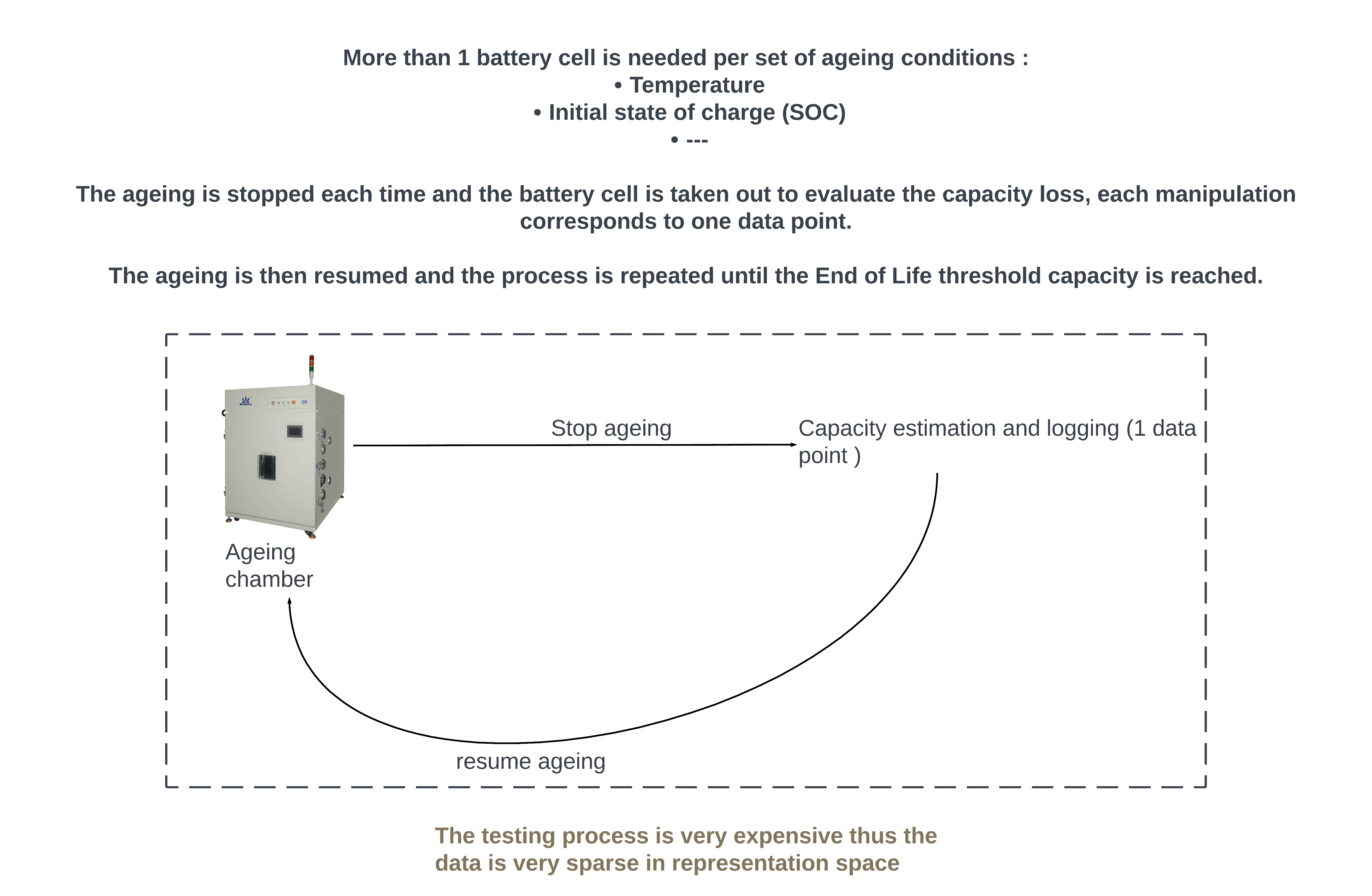
While widely used, such models often overlook manufacturing variations. Two batteries with identical specifications from different manufacturers can age differently, as observed in battery ageing tests conducted at Serma Technologies to gather a training dataset for our model.
Data collection
Limitations
- Expensive data collection resulting in sparse data, thus training a model using only experimental data would result in overfitting.
- Using the simple physics model doesn’t take into account the variance in factors like manufacturing processes.
Loss function
To address these challenges, we employed a novel approach, training a standard neural network (MLP) using a custom loss function taking into consideration the physics ageing equation as well as additionnal information from experimental data:
\[L_{training} = a_1 L_{MSE} + a_2 L_{DE}+a_3 L_{Boundary}+a_4 L_{CstPenalty}\]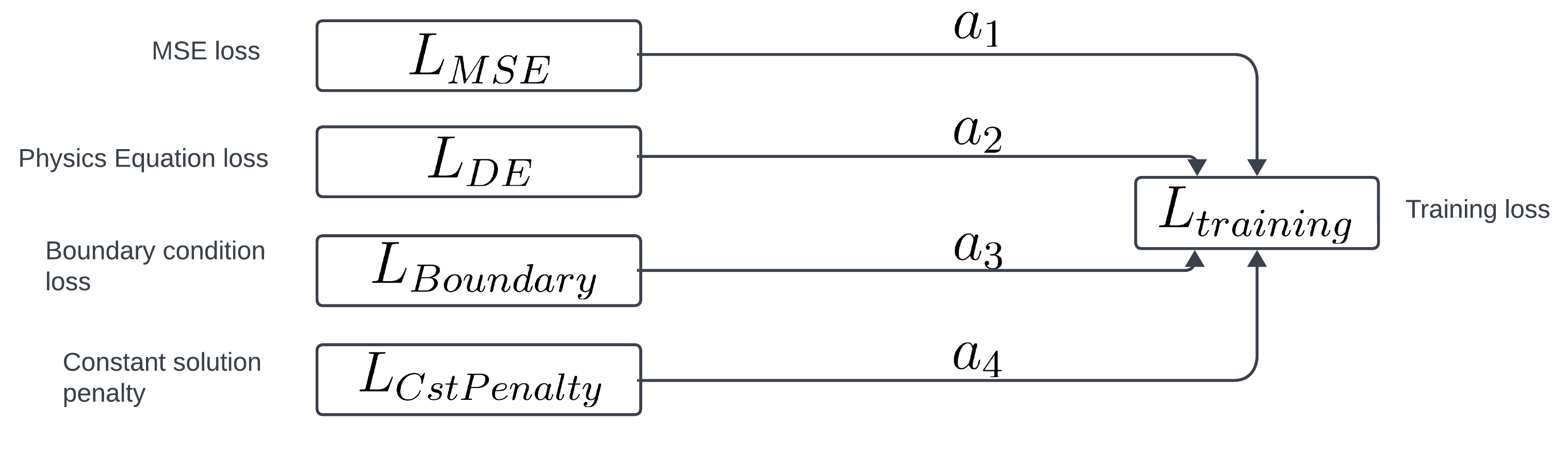
1- A general formulation of the Arrhenius equation:
\[\frac{\partial^2 C_{loss}}{\partial t}+\frac{1}{2t}\frac{\partial C_{loss}}{\partial t }=0\]The loss function derived from this equation:
\[L_{DE} = \frac{1}{n}\sum_{i=1}^{n} |\frac{\partial^2 f}{\partial t}(T_i,t_i,SOC_i;\theta)+\frac{1}{2t_i}\frac{\partial f}{\partial t }(T_i,t_i,SOC_i;\theta)|\]Where: f (T, t, SOC; θ) is the model’s response to the input (T, t, SOC) and θ the model parameters.
2- We also penalize the constant solution to the previous equation, so that the model doesn’t have a constant output which would minimize the $L_{DE}$ loss :
\[L_{CstPenalty} = \frac{1}{n}\sum|\frac{1}{\frac{\partial f}{\partial t}(T_i,t_i,SOC_i;\theta)}|\]3- MSE loss to learn from training samples : \(L_{MSE} = \frac{1}{n}\sum_{i=1}^{n}(f(T_i,t_i,SOC_i;\theta) - C_i)^2\)
4- A loss to translate the boudary condition, “no ageing at t=0” \(L_{Boundary} = \sum|f(T_{synth},0,SOC_{synth};\theta)|\)
PS: The coefficients $a_1$ , $a_2$ , $a_3$ , $a_4$ were tuned to balance the contribution of each loss and also the fact that the losses have different scales and to acheive convergence.
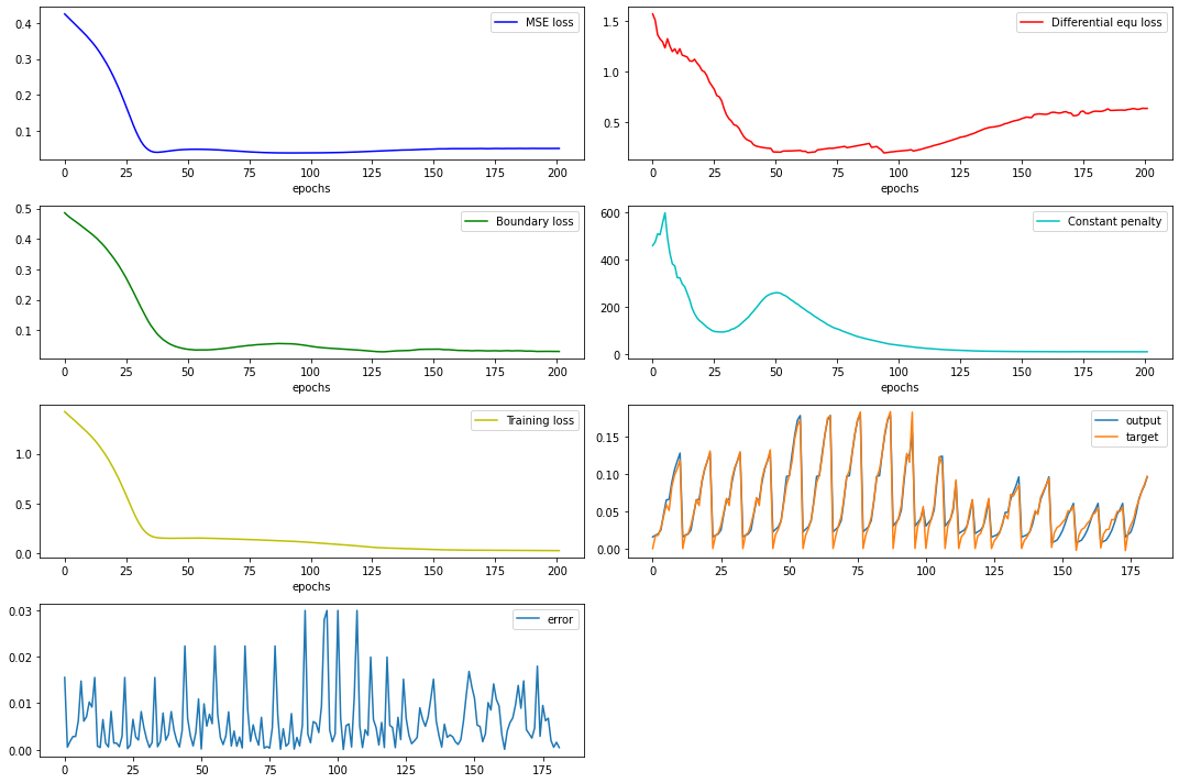
Training run
Results
- Improved mean absolute error on a batch of test cells from 1.05% (industry standard) to 0.38% (our method), a significant improvement in the context of the project.